
קובץ:Newton iteration.png
גודל התצוגה המקדימה הזאת: 729 × 599 פיקסלים. רזולוציות אחרות: 292 × 240 פיקסלים | 584 × 480 פיקסלים | 934 × 768 פיקסלים | 1,246 × 1,024 פיקסלים | 2,406 × 1,978 פיקסלים.
לקובץ המקורי (2,406 × 1,978 פיקסלים, גודל הקובץ: 55 ק"ב, סוג MIME: image/png)
| זהו קובץ שמקורו במיזם ויקישיתוף. תיאורו בדף תיאור הקובץ המקורי (בעברית) מוצג למטה. |
תקציר

|
קיימת תמונה חדשה תמונה זו בגרסה וקטורית בפורמט "SVG". יש להחליף את התמונה הנוכחית בתמונה החדשה.
File:Newton iteration.png → File:Newton iteration.svg
למידע נוסף אודות גרפיקה וקטורית, אנא קראו אודות המעבר של ויקישיתוף לתמונות בפורמט SVG. ראו גם מידע אודות התמידה של מדיה-ויקי בתמונות בפורמט SVG. |
 |
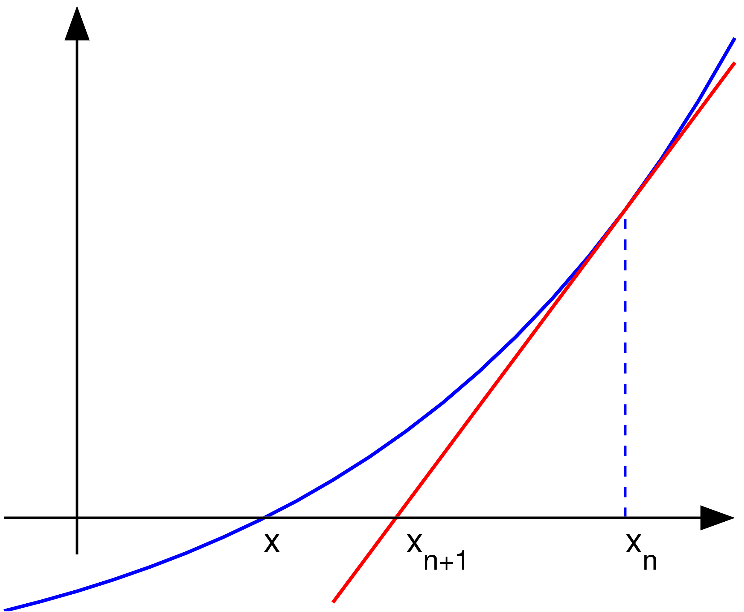
| תיאור | Uploader graphed this with en:MATLAB (Illustration of en:Newton's method) | ||
| תאריך יצירה | 22 בנובמבר 2004 (first version); 2004-11-23 (last version) | ||
| מקור | הועבר מ- en.wikipedia לוויקישיתוף. | ||
| יוצר | Olegalexandrov מוויקיפדיה האנגלית | ||
| PNGהתפתחות | MATLAB עם נוצרה ה PNG תמונת מפת סיביות | ||
| קוד מקור | MATLAB code
|
רישיון
| היצירה הזאת שוחררה לנחלת הכלל על־ידי היוצר שלה, Olegalexandrov מוויקיפדיה האנגלית. זה תקף בכל העולם. יש מדינות שבהן הדבר אינו אפשרי על פי חוק, אם כך: Olegalexandrov מעניק לכל אחד את הזכות להשתמש ביצירה הזאת לכל מטרה, ללא שום תנאי, אלא אם כן תנאים כאלה נדרשים לפי החוק. |
יומן העלאה מקורי
תיאור הקובץ המקורי נמצא כאן. כל שמות המשתמשים הבאים מתייחסים ל-en.wikipedia.
- 2004-11-23 19:55 Olegalexandrov 405×340×8 (14290 bytes) Scaled down the picture of Newton's method
- 2004-11-22 21:34 Olegalexandrov 509×406×8 (16510 bytes) I graphed this with Matlab (Illustration of Newton's method) {{PD}}
היסטוריית הקובץ
ניתן ללחוץ על תאריך/שעה כדי לראות את הקובץ כפי שנראה באותו זמן.
| תאריך/שעה | תמונה ממוזערת | ממדים | משתמש | הערה | |
|---|---|---|---|---|---|
| נוכחית | 06:23, 25 במאי 2007 | | 1,978 × 2,406 (55 ק"ב) | Oleg Alexandrov | {{Information |Description=Uploader graphed this with en:MATLAB (Illustration of en:Newton's method) ==Source code== <pre> <nowiki> % illustration of Newton's method for finding a zero of a function function main () a=-1; b=1; % interva |
| 02:11, 13 ביוני 2005 |  | 340 × 405 (6 ק"ב) | Everlong | optimized for smaller file size | |
| 02:06, 18 בינואר 2005 |  | 340 × 405 (14 ק"ב) | Andreas Ipp~commonswiki | {{PD}}: Original author graphed this with MATLAB (Illustration of Newton's method), from Wikipedia. |
שימוש בקובץ
![]() אין בוויקיפדיה דפים המשתמשים בקובץ זה.
אין בוויקיפדיה דפים המשתמשים בקובץ זה.
שימוש גלובלי בקובץ
אתרי הוויקי השונים הבאים משתמשים בקובץ זה:
- שימוש באתר en.wikipedia.org
- שימוש באתר fr.wikipedia.org