
קובץ:Aliasing between a positive and a negative frequency.png
אין גרסה ברזולוציה גבוהה יותר.
Aliasing_between_a_positive_and_a_negative_frequency.png (694 × 452 פיקסלים, גודל הקובץ: 44 ק"ב, סוג MIME: image/png)
| זהו קובץ שמקורו במיזם ויקישיתוף. תיאורו בדף תיאור הקובץ המקורי (בעברית) מוצג למטה. |
תקציר
| תיאור |
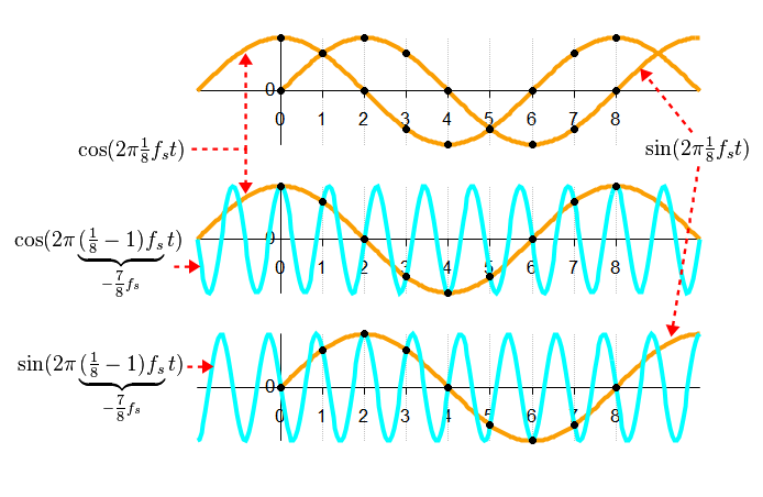
English: This figure depicts two complex sinusoids, colored gold and cyan, that fit the same sets of real and imaginary sample points. They are thus aliases of each other when sampled at the rate (fs) indicated by the grid lines. The gold-colored function depicts a positive frequency, because its real part (the cos function) leads its imaginary part by 1/4 of one cycle. The cyan function depicts a negative frequency, because its real part lags the imaginary part. |
|||
| תאריך יצירה | ||||
| מקור | נוצר על־ידי מעלה היצירה | |||
| יוצר | Bob K | |||
| אישורים והיתרים (שימוש חוזר בקובץ זה) |
אני, בעל זכויות היוצרים על עבודה זו, מפרסם בזאת את העבודה תחת הרישיון הבא:
|
|||
| גרסאות אחרות |
Derivative works of this file: Aliasing between a positive and a negative frequency.svg
|
|||
| PNGהתפתחות | LibreOffice עם נוצרה ה PNG תמונת מפת סיביות |
|||
| Octave/gnuplot source | click to expand
This graphic was created with the help of the following Octave script: graphics_toolkit gnuplot
gold = [251 159 3]/256; % arbitrary color choice
sam_per_sec = 1;
T = 1/sam_per_sec; % sample interval
dt = T/20; % time-resolution of continuous functions
cycle_per_sec = sam_per_sec/8; % sam_per_sec = 8 * cycle_per_sec (satisfies Nyquist)
figure
subplot(3,1,1)
xlim([-2 10])
ylim([-1.3 1.3])
% Plot cosine function
start_time_sec = -2;
stop_time_sec = 10;
x = start_time_sec : dt : stop_time_sec;
y = cos(2*pi*cycle_per_sec*x);
plot(x, y, "color", gold, "linewidth", 4)
box off % no border around plot please
hold on % same axes for next 3 plots
% Plot sine function
start_time_sec = 0;
stop_time_sec = 10;
x = start_time_sec : dt : stop_time_sec;
y = sin(2*pi*cycle_per_sec*x);
plot(x, y, "color", gold, "linewidth", 4)
% Sample cosine function at sample-rate (1/T)
start_time_sec = 0;
stop_time_sec = 8;
x = start_time_sec : T : stop_time_sec;
y = cos(2*pi*cycle_per_sec*x);
plot(x, y, "color", "black", ".")
% Sample sine function
y = sin(2*pi*cycle_per_sec*x);
plot(x, y, "color", "black", ".")
set(gca, "xaxislocation", "origin")
set(gca, "yaxislocation", "origin")
set(gca, "xgrid", "on");
set(gca, "ygrid", "off");
set(gca, "ytick", [0]);
set(gca, "xtick", [0:8]);
subplot(3,1,2)
xlim([-2 10])
ylim([-1.3 1.3])
cycle_per_sec2 = cycle_per_sec - sam_per_sec; % negative frequency
% Re-plot same cosine function on new axes
start_time_sec = -2;
stop_time_sec = 10;
x = start_time_sec : dt : stop_time_sec;
y = cos(2*pi*cycle_per_sec*x);
plot(x, y, "color", gold, "linewidth", 4)
box off
hold on
% Plot other cosine function
start_time_sec = -2;
stop_time_sec = 10;
x = start_time_sec : dt : stop_time_sec;
y = cos(2*pi*cycle_per_sec2*x);
plot(x, y, "color", "cyan", "linewidth", 4)
% Sample cosine functions at sample-rate (1/T)
start_time_sec = 0;
stop_time_sec = 8;
x = start_time_sec : T : stop_time_sec;
y = cos(2*pi*cycle_per_sec*x);
plot(x, y, "color", "black", ".")
set(gca, "xaxislocation", "origin")
set(gca, "yaxislocation", "origin")
set(gca, "xgrid", "on");
set(gca, "ygrid", "off");
set(gca, "ytick", [0]);
set(gca, "xtick", [0:8]);
subplot(3,1,3)
xlim([-2 10])
ylim([-1.3 1.3])
% Re-plot original sine function on new axes
start_time_sec = 0;
stop_time_sec = 10;
x = start_time_sec : dt : stop_time_sec;
y = sin(2*pi*cycle_per_sec*x);
plot(x, y, "color", gold, "linewidth", 4)
box off
hold on
% Plot other sine function
start_time_sec = -2;
stop_time_sec = 10;
x = start_time_sec : dt : stop_time_sec;
y = sin(2*pi*cycle_per_sec2*x);
plot(x, y, "color", "cyan", "linewidth", 4)
% Sample sine functions at sample-rate (1/T)
start_time_sec = 0;
stop_time_sec = 8;
x = start_time_sec : T : stop_time_sec;
y = sin(2*pi*cycle_per_sec*x);
plot(x, y, "color", "black", ".")
set(gca, "xaxislocation", "origin")
set(gca, "yaxislocation", "origin")
set(gca, "xgrid", "on");
set(gca, "ygrid", "off");
set(gca, "ytick", [0]);
set(gca, "xtick", [0:8]);
|


היסטוריית הקובץ
ניתן ללחוץ על תאריך/שעה כדי לראות את הקובץ כפי שנראה באותו זמן.
| תאריך/שעה | תמונה ממוזערת | ממדים | משתמש | הערה | |
|---|---|---|---|---|---|
| נוכחית | 08:26, 27 במרץ 2013 | | 452 × 694 (44 ק"ב) | Bob K | User created page with UploadWizard |
שימוש בקובץ
![]() אין בוויקיפדיה דפים המשתמשים בקובץ זה.
אין בוויקיפדיה דפים המשתמשים בקובץ זה.
שימוש גלובלי בקובץ
אתרי הוויקי השונים הבאים משתמשים בקובץ זה:
- שימוש באתר ms.wikipedia.org
- שימוש באתר sr.wikipedia.org