
קובץ:NonConvex.gif
אין גרסה ברזולוציה גבוהה יותר.
NonConvex.gif (360 × 392 פיקסלים, גודל הקובץ: 782 ק"ב, סוג MIME: image/gif, בלולאה, 84 תמונות, 4.2 שניות)
| זהו קובץ שמקורו במיזם ויקישיתוף. תיאורו בדף תיאור הקובץ המקורי (בעברית) מוצג למטה. |
The weighted-sum approach minimizes function


where


such that


To have a non-convex outcome set, parameters and are set to the following values


Weights and are such that


![{\displaystyle \omega _{1}\in [0;1]~}](https://wikimedia.org/api/rest_v1/media/math/render/svg/99c8913e84daf282e85b04849cc18cc14594dda7)

תקציר
| תיאור |
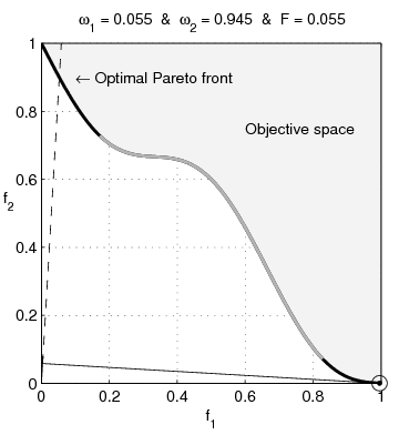
English: Weighted-sum approach is an easy method used to solve multi-objective optimization problem. It consists in aggregating the different optimization functions in a single function. However, this method only allows to find the supported solutions of the problem (i.e. points on the convex hull of the objective set). This animation shows that when the outcome set is not convex, not all efficient solutions can be found
Français : La méthode des sommes pondérées est une méthode simple pour résoudre des problèmes d'optimisation multi-objectif. Elle consiste à aggréger l'ensemble des fonctions dans une seule fonction avec différents poids. Toutefois, cette méthode permet uniquement de trouver les solutions supportées (càd les points non-dominés appartenant à l'enveloppe convexe de l'espace d'arrivée). Cette animation montre qu'il n'est pas possible d'identifier toutes les solutions efficaces lorsque l'espace d'arrivée est n'est pas convexe. |
| תאריך יצירה | |
| מקור | נוצר על־ידי מעלה היצירה |
| יוצר | Guillaume Jacquenot |
Source code (MATLAB)
function MO_Animate(varargin)
% This function generates objective space images showing why
% sum-weighted optimizer can not find all non-dominated
% solutions for non convex objective spaces in multi-ojective
% optimization
%
% Guillaume JACQUENOT

if nargin == 0
    % Simu = 'Convex';
    Simu = 'NonConvex';
    save_pictures = true;
    interpreter = 'none';
end

switch Simu
    case 'NonConvex'
        a = 0.1;
        b = 3;
        stepX = 1/200;
        stepY = 1/200;
    case 'Convex'
        a = 0.2;
        b = 1;
        stepX = 1/200;
        stepY = 1/200;
end

[X,Y] = meshgrid( 0:stepX:1,-2:stepY:2);

F1 = X;
F2 = 1+Y.^2-X-a*sin(b*pi*X);

figure;
grid on;
hold on;
box on;
axis square;
set(gca,'xtick',0:0.2:1);
set(gca,'ytick',0:0.2:1);

Ttr = get(gca,'XTickLabel');
Ttr(1,:)='0.0';
Ttr(end,:)='1.0';
set(gca,'XTickLabel',[repmat(' ',size(Ttr,1),1) Ttr]);

Ttr = get(gca,'YTickLabel');
Ttr(1,:)='0.0';
Ttr(end,:)='1.0';
set(gca,'YTickLabel',[repmat(' ',size(Ttr,1),1) Ttr]);

if strcmp(interpreter,'none')
    xlabel('f1','Interpreter','none');
    ylabel('f2','Interpreter','none','rotation',0);
else
    xlabel('f_1','Interpreter','Tex');
    ylabel('f_2','Interpreter','Tex','rotation',0);
end

set(gcf,'Units','centimeters')
set(gcf,'OuterPosition',[3 3 3+6 3+6])
set(gcf,'PaperPositionMode','auto')

[minF2,minF2_index] = min(F2);
minF2_index = minF2_index + (0:numel(minF2_index)-1)*size(X,1);

O1 = F1(minF2_index)';
O2 = minF2';

[pF,Pareto]=prtp([O1,O2]);

fill([O1( Pareto);1],[O2( Pareto);1],repmat(0.95,1,3));

text(0.45,0.75,'Objective space');
text(0.1,0.9,'\leftarrow Optimal Pareto front','Interpreter','TeX');

plot(O1( Pareto),O2( Pareto),'k-','LineWidth',2);
plot(O1(~Pareto),O2(~Pareto),'.','color',[1 1 1]*0.8);
V1 = O1( Pareto); V1 = V1(end:-1:1);
V2 = O2( Pareto); V2 = V2(end:-1:1);

O1P = O1( Pareto);
O2P = O2( Pareto);

O1PC = [O1P;max(O1P)];
O2PC = [O2P;max(O2P)];
ConvH = convhull(O1PC,O2PC);
ConvH(ConvH==numel(O2PC))=[];
c = setdiff(1:numel(O1P), ConvH);

% Non convex
O1PNC = O1PC(c);

[temp, I1] = min(O1PNC);
[temp, I2] = max(O1PNC);

if ~isempty(I1) && ~isempty(I2)
    plot(O1PC(c),O2PC(c),'-','color',[1 1 1]*0.7,'LineWidth',2);
end

p1 = (V2(1)-V2(2))/(V1(1)-V1(2));
hp = plot([0 1],[p1*(-V1(1))+V2(1) p1*(1-V1(1))+V2(1)]);
delete(hp);

Histo_X = [];
Histo_Y = [];
coeff = 0.02;
Sq1 = coeff *[0 1 1 0 0;0 0 1 1 0];
compt = 1;
for i = 2:1:length(V1)-1
    if ismember(i,ConvH)
        p1 = (V2(i+1)-V2(i-1))/(V1(i+1)-V1(i-1));
        x_inter = 1/(1+p1^2)*(p1^2*V1(i)-p1*V2(i));
        hp1 = plot([0 1],[p1*(-V1(i))+V2(i) p1*(1-V1(i))+V2(i)],'k');
        % hp2 = plot([x_inter],[-x_inter/p1],'k','Marker','.','MarkerSize',8)
        hp3 = plot([0 x_inter],[0 -x_inter/p1],'k-');
        hp4 = plot([x_inter 1],[-x_inter/p1 -1/p1],'k--');
        hp5 = plot(V1(i),V2(i),'ko','MarkerSize',10);

        % Plot the square for perpendicular lines
        alpha = atan(-1/p1);
        Mrot = [cos(alpha) -sin(alpha);sin(alpha) cos(alpha)];
        Sq_plot = repmat([x_inter;-x_inter/p1],1,5) + Mrot * Sq1;
        hp7 = plot(Sq_plot(1,:),Sq_plot(2,:),'k-');

        Histo_X = [Histo_X V1(i)];
        Histo_Y = [Histo_Y V2(i)];
        hp6 = plot(Histo_X,Histo_Y,'k.','MarkerSize',10);

        w1 = p1/(p1-1);
        w2 = 1-w1;
        Fweight_sum = V1(i)*w1+w2*V2(i);
        Fweight_sum = floor(1e3*Fweight_sum )/1e3;

        w1 = floor(1000*w1)/1e3;
        str1 = sprintf('%.3f',w1);
        str2 = sprintf('%.3f',1-w1);
        str3 = sprintf('%.3f',Fweight_sum);
        if (strcmp(str1,'0.500')||strcmp(str1,'0,500')) && strcmp(Simu,'NonConvex')
            disp('Two solutions');
        end
        title(['\omega_1 = ' str1 '  &  \omega_2 = ' str2 '  &  F = ' str3],'Interpreter','TeX');
        axis([0 1 0 1]);
        file = ['Frame' num2str(1000+compt)];
        if save_pictures
            saveas(gcf, file, 'epsc');
        end
        compt = compt +1;
        pause(0.001);
        delete(hp1);
        delete(hp3);
        delete(hp4);
        delete(hp5);
        delete(hp6);
        delete(hp7);
    end
end
disp(['Number of frames :' num2str(length(V1))]);
return;

function [A varargout]=prtp(B)
% Let Fi(X), i=1...n, are objective functions
% for minimization.
% A point X* is said to be Pareto optimal one
% if there is no X such that Fi(X)<=Fi(X*) for
% all i=1...n, with at least one strict inequality.
% A=prtp(B),
% B - m x n input matrix: B=
% [F1(X1) F2(X1) ... Fn(X1);
%  F1(X2) F2(X2) ... Fn(X2);
%  .......................
%  F1(Xm) F2(Xm) ... Fn(Xm)]
% A - an output matrix with rows which are Pareto
% points (rows) of input matrix B.
% [A,b]=prtp(B). b is a vector which contains serial
% numbers of matrix B Pareto points (rows).
% Example.
% B=[0 1 2; 1 2 3; 3 2 1; 4 0 2; 2 2 1;...
%    1 1 2; 2 1 1; 0 2 2];
% [A b]=prtp(B)
% A =
%      0     1     2
%      4     0     2
%      2     2     1
% b =
%      1     4     7
A=[]; varargout{1}=[];
sz1=size(B,1);
jj=0; kk(sz1)=0;
c(sz1,size(B,2))=0;
bb=c;
for k=1:sz1
    j=0;
    ak=B(k,:);
    for i=1:sz1
        if i~=k
            j=j+1;
            bb(j,:)=ak-B(i,:);
        end
    end
    if any(bb(1:j,:)'<0)
        jj=jj+1;
        c(jj,:)=ak;
        kk(jj)=k;
    end
end
if jj
  A=c(1:jj,:);
  varargout{1}=kk(1:jj);
else
  warning([mfilename ':w0'],...
    'There are no Pareto points. The result is an empty matrix.')
end
return;
. MATLAB עם נוצרה ה GIF תמונת מפת סיביות
רישיון
אני, בעל זכויות היוצרים על היצירה הזאת, מפרסם אותה בזאת תחת הרישיונות הבאים:

|
מוענקת בכך הרשות להעתיק, להפיץ או לשנות את המסמך הזה, לפי תנאי הרישיון לשימוש חופשי במסמכים של גנו, גרסה 1.2 או כל גרסה מאוחרת יותר שתפורסם על־ידי המוסד לתוכנה חופשית; ללא פרקים קבועים, ללא טקסט עטיפה קדמית וללא טקסט עטיפה אחורית. עותק של הרישיון כלול בפרק שכותרתו הרישיון לשימוש חופשי במסמכים של גנו. |
הקובץ הזה מתפרסם לפי תנאי רישיונות קריאייטיב קומונז ייחוס-שיתוף זהה 3.0 לא מותאם, 2.5 כללי, 2.0 כללי ו־1.0 כללי.
- הנכם רשאים:
- לשתף – להעתיק, להפיץ ולהעביר את העבודה
- לערבב בין עבודות – להתאים את העבודה
- תחת התנאים הבאים:
- ייחוס – יש לתת ייחוס הולם, לתת קישור לרישיון, ולציין אם נעשו שינויים. אפשר לעשות את זה בכל צורה סבירה, אבל לא בשום צורה שמשתמע ממנה שמעניק הרישיון תומך בך או בשימוש שלך.
- שיתוף זהה – אם תיצרו רמיקס, תשנו, או תבנו על החומר, חובה עליכם להפיץ את התרומות שלך לפי תנאי רישיון זהה או תואם למקור.
הנכם מוזמנים לבחור את הרישיון הרצוי בעיניכם.
היסטוריית הקובץ
ניתן ללחוץ על תאריך/שעה כדי לראות את הקובץ כפי שנראה באותו זמן.
| תאריך/שעה | תמונה ממוזערת | ממדים | משתמש | הערה | |
|---|---|---|---|---|---|
| נוכחית | 20:13, 8 במרץ 2009 | | 392 × 360 (782 ק"ב) | Gjacquenot | {{Information |Description={{en|1=Weighted-sum approach is an easy method used to solve multi-objective optimization problem. It consists in aggregating the different optimization functions in a single function. However, this method only allows to find th |
שימוש בקובץ
![]() אין בוויקיפדיה דפים המשתמשים בקובץ זה.
אין בוויקיפדיה דפים המשתמשים בקובץ זה.
שימוש גלובלי בקובץ
אתרי הוויקי השונים הבאים משתמשים בקובץ זה:
- שימוש באתר ar.wikipedia.org
- שימוש באתר az.wikipedia.org
- שימוש באתר de.wikipedia.org
- שימוש באתר el.wikipedia.org
- שימוש באתר en.wikipedia.org
- שימוש באתר pt.wikipedia.org
- שימוש באתר ru.wikipedia.org
- שימוש באתר sr.wikipedia.org
- שימוש באתר zh.wikipedia.org